Intuitive Understanding of GFlowNet
From first principles and makes you feel that you already know the algorithm.
Prerequisites:
- Basics of Directed Acyclic Graph (DAG)
- Basic Probability

And if you have read about GFlowNet before, then you would know that insights or terms from RL
are used in the algorithm. But to read this blog, you are not required to know RL.
Introduction
GFlowNet (Bengio et al., 2021) is an algorithm for sampling from an unnormalised discrete probability distribution over some compositional objects. Let’s first look at one of the applications and get some motivation about how such an algorithm can be helpful. In the case of drug discovery, the total number of compositional objects (drug molecules) can be exponentially large because different components (atoms) can be combined to form different objects (molecules). There are around \(10^{60}\) drug-like molecules. So, searching for the desired molecule takes time.
But we have a way to assign a score to each possible molecule, where a higher score means a molecule is potentially good. E.g., the binding affinity of a drug to a target protein can be considered a score where the higher the binding affinity, the better the drug molecule is. Because it can bind well with the target protein and do its work. This score can be considered as an unnormalised probability of a molecule after making it non-negative. And then we can try to sample from this distribution over molecules, where more molecules with higher scores should get sampled than the ones with lower scores. And the distribution is multimodal (because there are many molecules with higher scores), so we should also get a diverse set of potentially good molecules.
To sample from such a distribution, we need to find the normalisation constant, which would be difficult to compute because of the exponentially large number of objects. So, finding a way to sample from an unnormalised probability distribution is an important problem. There are many problems apart from drug discovery whose solutions can be framed as sampling from unnormalised probability distributions.
Many algorithms exist to do this, out of which the MCMC family is very popular. GFlowNet is a new algorithm for this task. A key quality of GFlowNet is that it can sample diverse objects because it can efficiently sample from different modes of the distribution. Now Generalised GFlowNet is also available, which can also sample from continuous distributions apart from discrete distributions.
By first hearing about GFlowNet, you may think this is another difficult AI algorithm, which has a steep learning curve. But when you try to understand it, there is a very intuitive understanding of it. Meaning, such intuitive understanding makes you feel that you already know all the pieces required to understand GFlowNet, it is just that you never combined these pieces.
These pieces are:
- Liquid flowing downward through a pipe network.
- A neural network
We know about neural networks as universal function approximators. And we also know how some liquid would flow through a pipe network.
Face Emoji Distribution
Now let’s take an example of an unnormalised probability distribution and then understand the GFlowNet through it. This is a very simplified version of the target distribution considered in Emmanuel Bengio’s Colab notebook. In this simple example, target distribution is the distribution over face emojis where a nose (left-pointed and right-pointed) is used instead of two eyebrows (as in the original example).
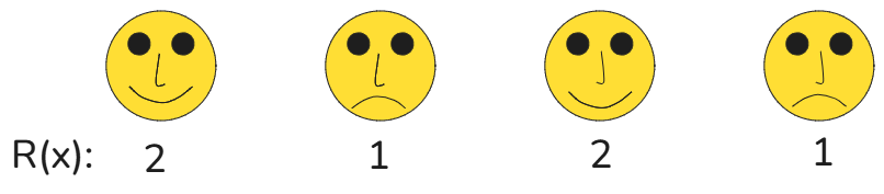
The unnormalised probability (the word “reward” will be used instead in the following sections, and hence the notation is \(R\)) of smiley faces is \(2\) and of frown faces is \(1\). So, smiley faces should get sample twice the number of frown faces.
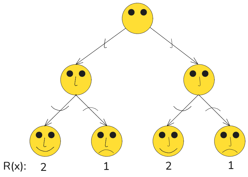
GFlowNet as DAG
We know about Directed Acyclic Graphs (DAGs), so first looking at GFlowNet as a DAG will be comforting. GFlowNet leverages the compositional nature of the objects to sample from a distribution. GFlowNet (“Net” here does not refer to a neural network but a different network, which will get clear in the following sections) is a DAG where intermediate nodes represent the incomplete objects. And leaf nodes represent the complete objects, which we want to generate or sample. There is only one root node. And an edge from node A to B represents an addition of some component to the incomplete object A to create a new object with that added component B. Then, the sampling process (or generation process) is nothing but “walking” on a “path” which starts from the root node and ends at a leaf node. At each node (including the root node), a probabilistic decision is taken to select the next outgoing edge, and the walk is continued through that edge. Reaching a leaf node means sampling the object corresponding to that leaf node. A leaf node can be reached via different paths, which means an object can be created in multiple ways.
Note:- In reality, intermediate nodes can also represent complete objects, depending on the application. E.g., in the molecule generation case, a small viable molecule can be part of a bigger viable molecule. So, an algorithm can decide to stop at the small molecule, or it can continue the walk and generate a bigger molecule from it. In this blog, in order to understand key concepts of GFlowNet easily, we are considering a simpler case, where only leaf nodes represent the complete objects (the objects which we want to sample). So, the unnormalised probability or reward of intermediate nodes will be zero.
GFlowNet as RL
Now, we have some sense of what GFlowNet is. Let’s now connect it with Reinforcement Learning (RL). Even if you do not know anything about RL, it is totally fine. This section is just about giving other names to the terms like ‘node’, ‘edge’, and ‘probabilistic decision’ already explained in the above section. And if you know RL, then you may understand the mechanisms of GFlowNet more quickly. Many of the notations (and concepts) used to explain GFlowNet come from RL, which we will define in the next section.
There is some similarity with RL or inspiration from RL where generation of an object (sampling process) is nothing but an agent in an environment, starting from a start state and taking a sequence of actions to reach a terminal state. Where each node of a DAG corresponds to a state and outgoing edges of a node correspond to the possible actions that can be taken in a state. The start state corresponds to the root node. And terminal states correspond to leaf nodes. And a probabilistic decision corresponds to an agent selecting an action by using a stochastic policy. By using a stochastic policy, an agent selects an outgoing edge at every node (excluding leaf nodes) while walking on a DAG, i.e., selects an action (which component to add) to take at each state. (For the ones who are familiar with RL, you may have already guessed from the previous section that the environment is deterministic, i.e., the next state is a function of the previous state and the action taken on it. Every time an action \(a\) is taken on the state \(s\), it will always lead to the same next state \(s^{\prime}\)).
So, many of the terminologies, like environment, policy, agent, action, and reward from RL, are used in the context of GFlowNet.
Notations
We have seen GFlowNet from the point of view of DAG and RL. So, each component of GFlowNet has two names coming from both these points of view. Before going ahead, let’s first define the notations which we will use from now on. As mentioned above, many of these notations come from RL.
Notations:
- The start state or root node is denoted by \(s_0\). The state at time zero.
- Any arbitrary state is denoted by \(s\) or \(s^{\prime}\).
- An action is denoted by \(a\).
- \(A(s)\) denotes the set of viable or allowed actions at state \(s\).
- A terminal state or a leaf node is denoted by \(x \in X\) where \(X\) is a set of complete objects.
- Probabilities, which are used to take probabilistic decisions at each node, are denoted by \(\pi\). It is called “policy” from the point of view of RL. To be more precise, \(\pi(a|s)\) denotes the probability of taking action \(a\) at state \(s\). Given state \(s\), the sum of probabilities of all the viable actions at \(s\) is \(1\). That is, there is a probability distribution over viable actions at a state which is given by the policy.
- The unnormalised probability of an object \(x\) is denoted by \(R(x)\) and it is called the “reward” for \(x\). The word “reward” for unnormalised probability will only make sense when you are familiar with RL. If you are not familiar with RL, then understand it as an agent getting some reward \(R(x)\) for sampling \(x\) according to some probability distribution. If an agent has to maximise the total rewards, then making unnormalised probability equal to rewards makes sense. If sampling according to this unnormalised probability distribution, objects with higher probability will get sampled more than others, which means the agent will receive a greater number of higher rewards than smaller rewards.
- A deterministic transition by taking action \(a\) at state \(s\) to the next state \(s^{\prime}\) (as explained above) is denoted by a function \(T(s, a) = s^{\prime}\).
There is also a third point of view (“GFlowNet as Flow Network” section), which will give a third set of names to the components of GFlowNet. But we will use the notations defined in this section.
Face Emoji Environment
Now that we know GFlowNet from the two points of view above. Let’s continue the face emoji example and start creating GFlowNet for it.
Environment determines how a DAG will be, i.e., what actions are allowed at each state and which next state each action at a state leads to (for the ones who are not familiar with RL, think of an open-world game. Where the world around a player is an “environment” where a player can’t fly, can only walk, and can’t buy if it is not near a store. If it walks forward (action), it will move forward (next state); if it sends (action) a dirty car to a car wash, it will receive a cleaned car (next state), etc.).
To create GFlowNet for face emoji distribution, the environment we consider is again the simplification of the environment considered in Emmanuel Bengio’s Colab (linked above). There are more restrictions (than in Emmanuel’s example) in the actions the agent can take given the state. In the start state, only two actions are allowed (no mouth actions) – a left-pointed nose or a right-pointed nose. And at the state with the nose, again only two actions are allowed – smile or frown mouth. Simplification is done so that we can find the policy easily by just looking at it and also to make the DAG small. Note that here we get a tree as a DAG.
GFlowNet as Flow Network
We have created a GFlowNet DAG for our face emoji example. To use it to do sampling, we need to find the appropriate policy for a given face emoji distribution. As mentioned above, the sampling process is nothing but walking on a path where, at each node, a probabilistic decision is taken. The policy at each node should be such that when multiple walks are taken, then number of walks ending at the \(x\) leaf node should be proportional to its reward \(R(x)\).
To understand:
- From a given unnormalised probability distribution \(R(x)\), how do you find the (appropriate) policy?
- And, by using this policy, how is sampling from such a distribution possible?
We will have to understand how creators of GFlowNet came up with this generative algorithm.
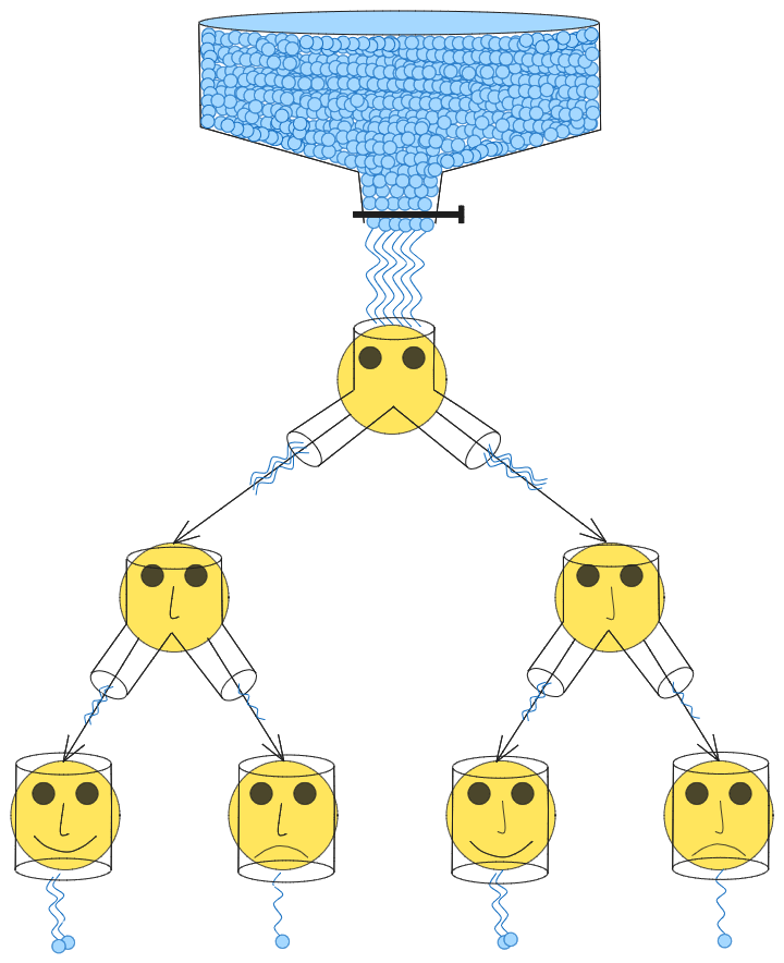
They came up with such an algorithm by taking inspiration from flow networks (e.g., a pipe network through which water is flowing). And hence the name Generative Flow Network (GFlowNet). The sampling process can be understood by looking at the DAG as a flow network. Visualise a pipe network corresponding to the DAG where edges are pipes and nodes are junctions. Each node junction has input openings and output openings. The number of input and output openings of a node junction equals to the number of incoming and outgoing edges of that node. With an exception, the root node junction has a single input opening, and leaf node junctions have a single output opening. Water enters into this DAG pipe network from the root node. So, there is a single entry point because there is only one root node. Gravity is such that water entering from the root node junction moves through the pipe network and gets out of the network via leaf node junction outputs. This is the direction of flow, unless specified otherwise. Gravity determines the direction of flow of water.
“Flow” in a pipe (edge) or junction (node) is nothing but the number of water molecules flowing through it. Flow of a pipe is denoted by \(F(s, a)\), and flow of a state or node junction is denoted by \(F(s)\).
Note:- Generally when the word “molecule” is used in the context of GFlowNet, it is used for molecules as target objects. But here, we are using water molecules (flowing through a pipe network) as an analogy to understand the workings of GFlowNet.
Now we have new terminologies for DAG components from the point of view of flow networks. Edges are called pipes, and nodes are called junctions (or called “node junction” to emphasise that they are just a node in a DAG). Flow division at a node junction through output openings is related to the policy.
Let’s state two conditions the pipe network should follow so that understanding GFlowNet through it becomes intuitive:
-
The root node junction is connected to a water tank with a valve. When the valve opens for a time period \(t\), some \(Z\) number of molecules (let’s call it a “batch” of molecules) move from the tank into the pipe network. They move through the pipe network and get out of it via its leaf node junctions. The number of water molecules entering the network should be equal to the number of water molecules getting out via all leaf node junctions (there is no leakage). Which means input flow=output flow at all intermediate junctions \(s^{\prime}\):
\[\sum\limits_{s,a:T(s,a)=s^{\prime}} F(s, a) = \sum\limits_{a^{\prime}\in A(s^{\prime})} F(s^{\prime}, a^{\prime}) = F(s^{\prime})\]and,
\[Z = \sum\limits_{a\in A(s_0)} F(s_0, a) = F(s_0)\] -
Each node junctions first collects all flows from its incoming edges, then shuffles the collected water (total inflow) randomly, then divides it and flows it out through output openings of these node junctions. This division (outgoing edge flow assignment)
\[F(s) = \sum\limits_{a\in A(s)} F(s, a)\]at each node junctions \(s\) (with multiple outgoing edges) should be such that flow getting out of \(x\) leaf node should be equal to its reward \(R(x)\), which implies:
\[Z = \sum\limits_{x\in X} R(x)\]Different node junctions may divide their total inflow differently. Assigning some flow to an edge means adjusting the pipe width and cross-sectional area of corresponding openings to which it is connected. So that when water flows naturally (in gravity’s direction), it gets divided at each junction according to these assigned edge flows. The more the cross-sectional area, the more water should flow through it, so edge flow is directly proportional to its corresponding cross-sectional area.
Flow Network Sampling Process
Building the generative or sampling algorithm from analogy with a conditioned flow network (a flow network that follows the above two conditions) is easy. Let’s first see how one can sample from a given unnormalised distribution \(R(x)\) with the help of a conditioned flow network. The sampling process via conditioned flow network is like this:
- Open a valve for period \(t\).
- Choose one of the \(Z\) molecules in a batch uniformly (all molecules are equally likely to get chosen).
- Track it and find out through which leaf node that molecule gets out.
- Then the object corresponding to that leaf node through which it gets out is the generated object or sampled object.
Let’s call this sampling process the “Flow Network Sampling Process” (in short, the FN sampling process). When you repeat this process again and again, let’s say \(Z\) times, then you will immediately understand how objects will get sampled proportional to their rewards.
Why? Because you know all \(Z\) molecules will come out via leaf nodes (first condition) and the outflow of the \(x\) leaf node equals to its reward \(R(x)\) (second condition). And we could have chosen any of the \(Z\) molecules that come out via one of the leaf nodes. It means if we repeat the FN sampling process, let’s say \(Z\) times (i.e., choosing a total of \(Z\) molecules and generating \(Z\) number of objects or creating \(Z\) samples). Then in an ideal case, number of chosen molecules (out of \(Z\)) comes out via \(x\) leaf node will be \(R(x)\). In a non-ideal case, number of chosen molecules coming out of \(x\) leaf node may not be exactly \(R(x)\). But in the long run of repeating the FN sampling process let’s say \(100Z\) times, number of chosen molecules (out of \(100Z\)) coming out of \(x\) leaf node will be more or less \(100R(x)\), which means proportional to \(R(x)\).
This sampling process depends on the two conditions above. One can think of ensuring the first condition of no leakage easily. But what about the second condition? How to divide the flow at all junctions with multiple output openings (i.e., how to adjust the cross-section of output openings of all such junctions or how to do outgoing edge flow assignment)?
One naive way is this. To do outgoing edge flow assignment simply means to know the appropriate edge flow for all the edges. What we have are the desired flows (i.e., rewards \(R(x)\)) of all the leaves. So, given these desired leaf flows, let’s find the appropriate edge flows. Let’s pick a leaf node \(x\). To receive the desired flow \(R(x)\) at this leaf, this much flow must come from its incoming edges, which means there is no restriction about how to divide the total flow \(R(x)\) into its incoming edges. So, divide arbitrarily and assign the flows to its incoming edges. Now repeat this process for all the leaves. Now there will be a set of nodes (nodes which are only directly connected to leaves) for which we know outgoing edge flows of each node in the set. Now calculate the flow of each node in this set by simply adding their outgoing edge flows. Now repeat the above process of arbitrarily assigning incoming edge flows for all the nodes in this set. Based on this idea, here is the algorithm to calculate appropriate edge flows for all the edges:
Naive Edge Flow Assignment Algorithm – Iterate until we calculate the flow of all edges. In each iteration, do this:
- Arbitrary incoming edge flow assignment: Create a set \(S\) which contains all the nodes whose flows we know but do not know their incoming edge flows. Iterate over this set. In each iteration \(i\), arbitrarily distribute the flow of node \(s^i\) and assign it to its incoming edges.
- Node flow calculation: Now there will be some set of nodes whose outgoing edges got assigned some flows. So, now calculate the flow of each such node by simply adding their outgoing edge flows.
Face Emoji Flow Network
Let’s now create a corresponding flow network of the emoji DAG and also apply the above two conditions. According to the rewards assigned above to each leaf node, the total number of water molecules that should flow through the pipe network is 6 (summation of rewards of all leaf nodes). In the diagram, the flow of a single water molecule is represented via a wiggly line. The diagram also shows the division of water flow at each junction such that the number of molecules getting out of the leaf node equals to the reward of that leaf node. Here we do not even need the naive edge flow assignment algorithm. We can assign edge flows by just looking at the DAG. We can calculate edge flows like this in such simple examples where the DAG is small.
In the real, complex distributions, finding the exact edge flows would be computationally expensive via the naive edge flow assignment algorithm, but we can leverage deep learning and can find a good flow approximator function cheaply. But before we look at it, let’s first see how we can make a sampling algorithm if we know all edge flows in a flow network.
Sampling Algorithm from Flow Network
We looked at the sampling process from the view of the pipe network and water flow. But how can we simulate this process in a computer, i.e., how do we convert this understanding of sampling via water flow to a computer algorithm so that we can actually do the sampling and not just visualise or imagine it in our head?
If we naively convert this into an algorithm, then we would need to do fluid simulation. But there is one other cheap way of tracking the chosen molecule by relying on the fact that each junction randomly shuffles the collected water (from incoming edges) before dividing or distributing it to outgoing edges.
Which means a chosen molecule at a node will select an outgoing edge probabilistically (because of shuffling), and this probability is independent of the incoming edge it arrived from (again, because of shuffling).
After shuffling, the probability that a chosen molecule will go through an outgoing edge (or pipe) is directly proportional to its cross-sectional area. The larger the cross-sectional area, the greater the chance that a chosen molecule will lie near it after shuffling. And as explained above in the second condition, the cross-sectional area of an outgoing pipe (or edge) is directly proportional to its flow.
Therefore, at each node \(s\) with multiple outgoing edges, a chosen molecule coming from anyone of the incoming edges will go through anyone of the outgoing edges \(a\) according to this probability:
\[P(a|s) = \frac{F(s, a)}{\sum\limits_{a^{\prime}\in A(s)} F(s, a^\prime)}\]If we know all edge flows, then we can calculate these probabilities for all the nodes (with multiple outgoing edges). Knowing the probability distribution over outgoing edges means we can sample from it. Which means we can track a chosen molecule in a pipe network (FN sampling process) by sampling the outgoing edge at all the nodes starting from the root node until we reach the leaf node. This is exactly what walking on a path over a DAG is (as mentioned in the “GFlowNet as DAG” section). Therefore, policy (which we didn’t know until now) is nothing but the probability mentioned above, calculated via edge flows:
\[\pi(a|s) = P(a|s)\]So, with the help of analogy with the flow network, we not only calculated the policy but also understood how sampling from a given unnormalised probability distribution is possible by following this policy while walking on a path over a DAG.
Training
Now we know that we can sample according to a given unnormalised probability distribution if we know the appropriate edge flows. And by using the analogy with a pipe network, we also know that flow can be appropriately divided at each junction, i.e., appropriate edge flows exist. We looked at one naive way of finding the appropriate edge flows, but it is not efficient when our DAG is exponentially large (e.g., in the case of drug generation).
In GFlowNet, edge flows are calculated by training a neural network (with parameters \(\theta\)) to map the state or node to a vector containing appropriate outgoing edge flows.
Training is done via flow-matching loss applied over intermediate states and terminal states. Loss w.r.t. an intermediate state \(s^\prime\) is:
\[L(s^\prime) = \Bigg(\sum\limits_{s,a:T(s,a)=s^{\prime}} F_{\theta}(s, a) - \sum\limits_{a^{\prime}\in A(s^{\prime})} F_{\theta}(s^{\prime}, a^{\prime})\Bigg)^2\]And for all leaf nodes \(x\in X\), loss is:
\[L(x) = \Bigg(\sum\limits_{s,a:T(s,a)=x} F_{\theta}(s, a) - R(x)\Bigg)^2\]Because outflow of a leaf node should be equal to its reward.
In the original GFlowNet paper, loss for all the states is defined via the single equation. To have such a single definition for loss, we have to assume that allowed action sets for all terminal states are null: \(A(x)=\phi\) for all \(x\in X\). Which means there are no outgoing edges from leaves, but above, we mentioned that there is a single outgoing opening at each leaf node junction, so to respect this, we wrote separate losses for terminal and intermediate states.
Global minima with zero loss is achieved when flow matches at all the states. We know zero loss is possible because we know that the corresponding flow network with appropriate edge flows exists. And we know that a neural network with sufficient size is an universal approximator, and a global minima can be reached if trained longer.
We want to evaluate the neural network on the training data (states or nodes of a DAG) itself, so there is no problem of overfitting. But there is a problem of underfitting because in real-world applications like molecule generation, DAG will be exponentially large, so there will be a huge amount of training data, and it would take time to train on all nodes.
Code
Using the code from Emmanuel Bengio’s Colab on emoji GFlowNet but with one tweak in how loss is calculated. This code creates GFlowNet for the original face emoji distribution used in the Colab, but full-batch loss is used rather than mini-batch loss.
Mini-batch loss in the case of GFlowNet training is atypical because it requires sampling in the training loop. So to make the training pipeline more familiar for beginners, full-batch loss is used. In the full-batch loss case, all the possible states are first stored in a dictionary before training. Then in every epoch, loss w.r.t. each state in a dictionary is calculated, and final loss is calculated by adding all these state losses.
Here is the link to the repo: https://github.com/joshi98kishan/understanding_gflownet
Conclusion
We have seen GflowNet from multiple points of view: DAG, RL and flow networks. With the help of the “water flowing in a pipe network” analogy, we calculated the appropriate policy and also intuitively understood how GFlowNet can sample from unnormalised probability by following this policy. We also created a GFlowNet for the simplified face emoji distribution. And saw simplified code (using full-batch loss) for original face emoji distribution.
After going through this blog, some questions may still remain, which we may cover in detail in future blogs:
- Difference between RL and GFlowNet? In short, the key difference between RL and GFlowNet is that RL tries to find the policy such that reward gets maximised. While GFlowNet tries to find a policy such that it can sample according to the distribution given by rewards.
- Why can’t we have a single node (with the number of outgoing edges equal to the total number of unique objects in a given distribution) instead of a graph? The short answer is that calculating the normalisation constant is computationally expensive for real-world distributions like distributions over molecules.
- How does GFlowNet make this sampling process or approximation of the normalisation constant easy compared to other such algorithms like MCMC?
Learning Resources
- The GFlowNet Tutorial by Yoshua Bengio, Kolya Malkin, and Moksh Jain.
- Introduction to GFlowNets - Part 1 - Emmanuel Bengio YouTube video.
- Colab notebook by Emmanuel Bengio already mentioned above.
Thank you for reading. Feel free to email me for any corrections.